Two Pulsar Discoveries by Anna H. '14

In 1965, Jocelyn Bell arrived at Cambridge University to earn her Ph.D. Two years later, she found herself working with four other people to string up 120 miles of wire and cable and set up over 1000 posts: they built a radio telescope that could fit 57 tennis courts. Bell was put in charge of operating the telescope, and collecting data. Bear in mind that you can’t just stick your eye into a radio telescope; nowadays, astronomers “see” using digital electronics magic, but back in 1967 Bell was stuck using a pen chart recorder. It spat out a hundred feet of paper per day, which she analyzed by hand, because she was (and is) a beast.

A few months after first light, Bell noticed some strange noise. Most of us think of “noise” as unwanted sound – in astronomy, it’s the same thing, except we’re dealing with light waves instead of sound waves. Noise is signal from sources a) here on Earth, that interfere with what’s coming at us from space, or b) out in space, that aren’t what we’re intending to look at . Basically, it’s extraneous, hard to get rid of, and the most annoying thing ever. It’s why the area around the Green Bank radio telescope in West Virginia (where my data is collected) is a National Dark Zone: no electronics equipment allowed. No spark plugs. If you want to drive up close, you have to use a car that runs on diesel. There are some old school machines out there.

Fortunately for the scientific community, Jocelyn Bell paid special attention to the noise that she saw, instead of discarding it. She paid attention because the noise took a strange form: little pulses, spaced precisely one and a third seconds apart. She told her supervisor, and they figured that something so regular had to be man-made. Since it had to be man-made, it had to be coming from Earth. Something from Earth was interfering with the signal. Great.

Then Bell noticed that, every day, the whole pulsing sequence was delayed by four minutes. “Delayed by four minutes every day” is a familiar expression to astronomers. One day, to us on Earth, is defined as the time it takes for the Sun to reappear in the same place in the sky. As Earth rotates, it’s also traveling in orbit around the Sun, which causes the Sun to take four minutes longer each day to reappear in that same place. So, our “day” is actually one full Earth rotation, plus a little bit extra. Essentially, the fact that Bell’s noise was getting delayed by four minutes every day meant that it wasn’t coming from Earth: it was coming from the stars. From space.

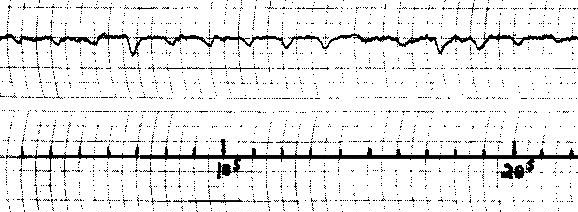
Those little blips up top are the noise that Bell saw. 

So. We have a regular signal, which is surely artificial, coming from space. Naturally, this means: ALIENS! The source was named LGM-1: Little Green Men 1.

…

Right. You probably realize by now that if this post was about the 1967 discovery of extraterrestrial intelligence, it would be old news to you. This post is NOT, in fact, about aliens: Bell’s “noise” turned out to mark the discovery of pulsars. A pulsar is the tiny (~12km radius) super-dense spinning remnant of a star that has gone supernova; because of its magnetic field (it’s basically a spherical spinning bar magnet) it emits a narrow beam of radiation. As it spins, the beam flashes past Earth, exactly like a lighthouse, which is why we only receive little signal blips, and why it appears to “pulse”.

Since 1967, the search has been on for more pulsars. There are currently about 1600 pulsars known, 34 of which live in a globular cluster called Terzan 5. I’m particularly attached to Terzan 5, because it’s home to the pulsars that I do my research on. Finding a pulsar is not easy, for a few reasons. For one, pulsars are tiny: city-sized, or smaller. For another, their signal is very VERY weak compared to most of our other radio sources. If we just pointed a telescope up at the sky and looked at the data, the pulsar’s signal would be there somewhere, but it would be buried underneath noise and other ickiness.

To deal with this, we use a technique called “folding.” I think it’s pretty ingenious, so bear with me for a couple of paragraphs and a couple of pictures (or skip to the end of the post, if you want to get straight to the punchline.)

Raw data looks something like this:

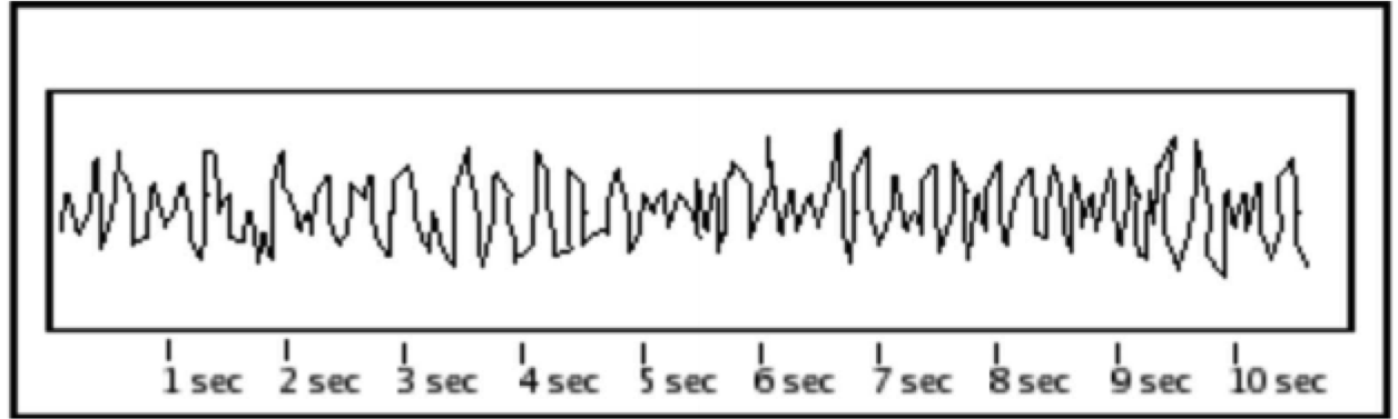
Basically, you have some signal that varies over time. This looks like garbage – there’s no obvious pulsar signal in that image. There might be one hidden, there might not be. How do we draw it out? Imagine that we could somehow guess the pulsar’s period (the length of time between pulses). Imagine that we knew it was 1 second. We could mark up the piece of paper like this:

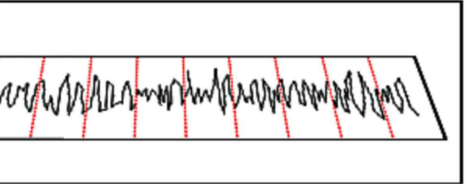
Because the pulse appears EXACTLY once a second, and we’ve marked up the paper into second-long chunks, we know that the signal must appear exactly once in each chunk. Not just that – it must appear in exactly the same place in each chunk. Now, we take a pair of scissors to the data, slice it up along the red dotted lines, and stack the sections on top of each other – in other words, we fold it.

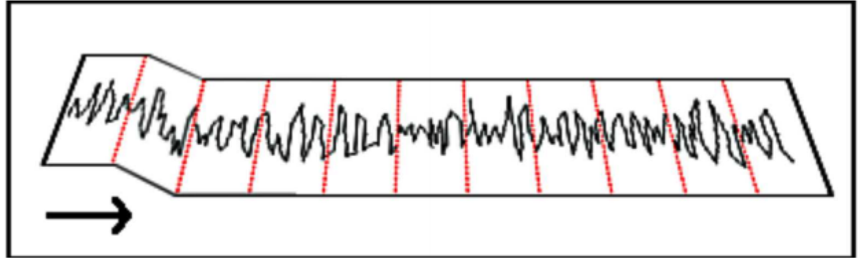
The signal from all those stacked slices is added up. Because the pulsar signal appears at exactly the same position in each slice, the total signal gets stronger and stronger as you add up more and more slices. Other stuff, like noise and interference, probably doesn’t appear at exactly the same place in every second-long data slice: it doesn’t add up. It cancels itself out, maybe, or averages out to a much lower value. The pulsar’s signal, though, shines through, and we get something like this:

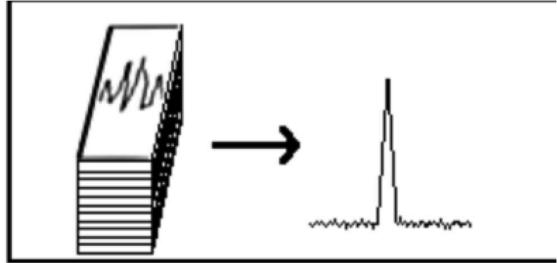
Bam. Pulsar. Of course, our data nowadays doesn’t come on a long strip of paper. If I took a pair of scissors to my data and tried to stack it up by hand, I wouldn’t finish in my lifetime (and there’s other stuff I’d rather be doing, to be honest.) I deal with terabytes of data, and get big computer clusters to “fold” it for me. When it finishes, I take a look at the result of the stacking – the sum of all the signal – and see whether I’ve found a pulsar.

This is the kind of plot I look at:

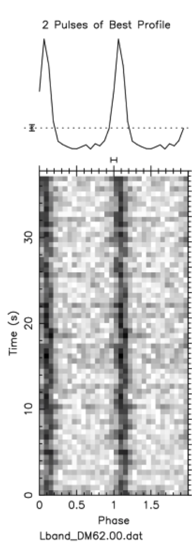
Look closely, and you’ll see that the image is made up of lots of tiny white, grey, and black squares. One row of those little squares corresponds to one slice of paper: what you get after you cut up the whole strip. The whole column is the “sum” of all those slices of paper – we’ve stacked them, exactly like in the paper analogy. The “pulse profile” at the top is the sum of all the pulses.

Below is a plot of…almost exactly the same thing. Before you go on to read my explanation of what it is, try to figure it out.

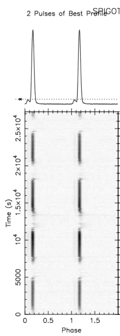
It’s an eclipsing binary pulsar! Basically, the pulsar is in a binary system with a star (usually a white dwarf), and periodically gets “eclipsed” by its companion. It’s cool when what you see perfectly matches what you would predict.

So, now you know how to find a pulsar. In practice, it’s a little more complicated than this – there are other factors like dispersion and rotation of the EM beam that I didn’t go into. What I just described is the essential part, though. And now, for another story of pulsar discovery:

As a side project (I’ll describe my main project in another post) I’ve been doing some pulsar searching. This takes a completely different form from what J. Bell was doing. Basically, I run a bunch of Python scripts in the terminal, and check the plots they spit out to see whether I’ve found a pulsar. My supervisor has a bunch of new, high-quality data, so I have a lot to search through. It takes a long time to do the “folding”, because (like I mentioned earlier) we’re dealing with ridiculous amounts of data. So, one night during my second week of work, I set up a bunch of folds to run overnight, and went home. I got into the office in the morning, eager to see the results – and saw a bunch of error messages on my screen. Some Unix stuff that was gibberish to me.

NOOOOOOOOOOOOOO!!!!

I sent an e-mail to my supervisor, explaining that something had gone wrong (although I wasn’t really sure what) and that I would re-run the folds that day. In the meantime, all sad and disheartened, I restarted the folds. About half an hour later, my supervisor walked into the room, beaming at me.

Supervisor: Hey-
Me: AHHHHHHHHH I CAN’T BELIEVE IT CRASHED! I’M SO HEARTBROKEN!
Supervisor: I-
Me: I THINK IT RAN OUT OF PROCESSING SPACE IT SAID IT WAS OUT OF MEMORY
Supervisor: Well,-
Me: DON’T WORRY I STARTED IT AGAIN HOPEFULLY IT’LL BE READY SOON
Supervisor: All the files are there.
Me: IT MIGHT TAKE ANOTHER FEW HO-what?
Supervisor: The process finished. The files are there.
Me: WHAT?
Supervisor: Yup! I checked. They’re all there.
Me: I-what? Why did it say it ran out of memory?
Supervisor: It just wasn’t able to actually load the images.
Me: Oh! Sweet. Wait. WAIT. That means the files are on there???
Supervisor: Yup!
(Part of the problem was that it put the files in a place I didn’t expect.)

My hands were shaking so hard that I messed up the command line over and over again (my supervisor was, fortunately, very patient) – and then it appeared! The Plot.

This plot:

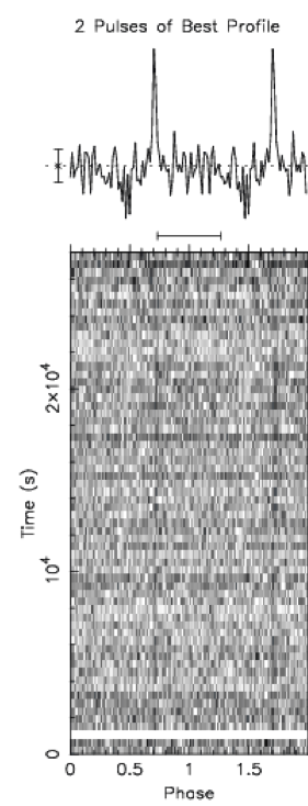
The signal isn’t as obvious as in the sample plots I showed you…but it’s there. Two dark lines running down the time/phase block, and the clear pulse profile. A new pulsar, that no one has ever seen before. His name is Terzan5aj, and if *actually* confirmed (he has “very likely” status – we have to find him in some other observations in order to be 100% sure), he will be the 35th and faintest pulsar ever found in Terzan 5. That, plus the fact that he probably has significant scintillation going on (he’s brighter at some times than others…basically, he twinkles through the intergalactic medium, like a star) is why he escaped notice before. There is now a picture of him (more specifically, four graphs of his behaviour) on my wall.

I should mention that this “discovery” has very little to do with me, in the sense that all I did was run a bunch of Python scripts on brand new fancy shmancy data collected by my supervisor. But still. I was the first person to ever see that pulsar. And for MILLENNIA after I’m gone, he’ll still be spinning at >700 times per second. And that’s pretty cool.