Hilbert’s Third Problem (A Story of Threes) by Lydia K. '14, MEng '16
Holy mathematics, Batman! Math at MIT, and why we need calculus to define volume.
18.304 (discrete math) is one of two communication intensive (CI-M, where the M means it’s within my major) seminars I need to take as part of my math major. (The second one, which I’m taking this semester, is 18.424, information theory. The other seminar topics we get to choose from are
- real analysis,
- analysis,
- discrete applied mathematics,
- physical mathematics,
- theoretical computer science,
- logic,
- algebra,
- number theory,
- topology, and
- geometry.)
The math CI-Ms are small classes, taught almost entirely by the students: in my experience so far, after a few starter lectures by the professor every student presents three lectures as a combination of slide presentations and chalktalks. Sometimes there are also p-sets; sometimes there are not. At the end of the semester we write in-depth explorations of the topics of our final presentations.
In 18.304, I got to transiently experience several dozen proofs, getting closely acquainted with two of them and reading books and books and books about a third. My first topic was Dijkstra’s algorithm for finding shortest paths, my second topic was (the inifinite-ish quantity of) proofs for the infinity of primes, and my third topic was Hilbert’s third problem, which we’ll get to know much more closely in this blog post. The first two presentations went objectively horribly. The third one went much better: I showed up early and stood in front of the bathroom mirror similing to myself for 20 seconds in a Wonder Woman power pose. On the way from the bathroom to the classroom I passed a girl from among my soon-to-be audience. We made eye contact and exchanged shy smiles and somehow that made everything better: I felt less alone, and I felt that I had an ally among the people I had been scared were going to judge me. (If you’re reading this, thank you so much, kind, mysterious friend-when-I-needed-one.)
Over the course of the semester, I went from having barely any exposure to proofs beyond what I’d gotten from my computer science classes and general institute requirements to being able to follow, read, write, and (thanks to 6.046, which I took at the same time) formulate a proof. This was a huge amount of growth for me, and a big part of my goal in becoming a math major.
My grandfather, who was very, very dear to me, emphasized to me that there is a lot of power at the intersection of fields. It is valuable to be able to be a translator between fields, to be an avenue for the ideas, tools, and strengths of one field to enter and innovate in another field. This has been one of my hopes for my technical education at MIT: as a 6-7/18 major, I’m split officially between three technical departments—computer science, biology, and mathematics—and I’ve also had to take courses in physics and chemistry. My personal theory (and experience) is that computational biology, the thing I am ultimately studying, is young enough that depending on their backgrounds, people primarily approach it from the perspective of biology, computer science, or math—occasionally two of them, but very rarely all three. I’m hoping that my broader education at MIT will help me find a niche and be, as my grandfather said, a useful translator across those junctions.
The rest of this blog post is my final paper, which from the very start I wrote with the dual purpose of turning in and posting here, with an intended audience of high school students. (Feel free to skim or skip around if it helps you get a picture of the proof.) I’m hoping to write a post about Dijkstra’s algorithm someday as well, since it is one of my favorite algorithms (tied maybe with Edmonds-Karp, because flow networks are absurdly useful).
I want to communicate the following things I have learned about math:
- Math is an incredibly diverse field, not a single path, and you may or may not have gotten a chance to actually see all the many branches in high school.
- Math is a human and even political field, in which a single problem can connect people across centuries.
- Math is not memorization—in fact, the human subject of this blog post chose math specifically for that reason.
1 Introduction and History
Hilbert’s third problem, the problem of defining volume for polyhedra, is a story of both threes and infinities. We will start with some of the threes. Already in early elementary school we learn about two- and three-dimensional shapes and some of their interesting properties. We learn that a triangle is a two dimensional polygon with three edges.
More generally, we learn that a polygon can be defined as a two-dimensional shape constrained to a plane, bounded by any number of straight, uncurved lines, the edges. The area contained between the edges is the single face of the polygon and the points where the edges meet are the vertices.
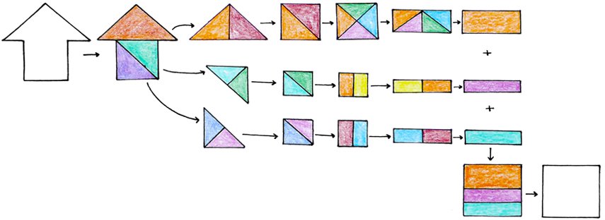
All polygons can be cut up into a discrete number of triangles, and the area of these triangles can always be further distributed in discrete chunks to form a square of the same area as the original polygon. One method of doing this is to cut the polygon up into triangles, cut each triangle up into smaller triangles that can be reassembled into a rectangle, and cut this rectangle up and rearrange the pieces into another rectangle, this one with either its width or its height equal to the side length of the square we want to assemble. Finally, we can stack these rectangles to form a square with the same area as our original polygon, a square shared by all polygons of that area.
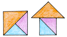
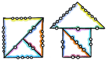
As an example, here we chop up a two-dimensional house and rearrange it into a square of the same area.
1.1 Definition I: Equidecomposable
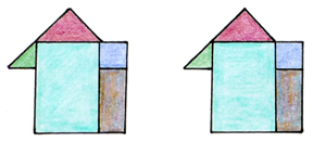
The ability to chop up one figure and build a new one out of its pieces is the first property we are interested in: equidecomposability. Two shapes are equidecomposable if they can be divided up into congruent building blocks. For example, the house and the square that we looked at above are equidecomposable. Below is another of the many ways that they can be decomposed into congruent pieces.
This relationship can be expressed mathematically. In the picture above, both the square S and the house H can be decomposed into the orange (O), purple (P), and blue (B) pieces.
S = O ∪ P ∪ B = H
Equidecomposability has also been called congruence by dissection and scissors congruence.
1.2 Definition II: Equicomplementable
Another property that we are interested in is equicomplementability. Two shapes are equicomplementable if congruent building blocks can be added to both of them to create two equidecomposable supershapes. In addition to being equidecomposable, our house and square are also equicomplementable.
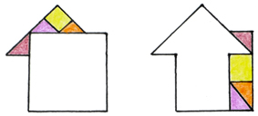
The supershapes we have created are equidecomposable.
We can express this relationship mathematically as well. We can add four pieces—here a yellow piece Y, a pink piece P, an orange piece O, and a maroon piece A—to the square S in order to create a supershape M. We can add the same pieces to the house H to create a second supershape N.
M = S ∪ Y ∪ P ∪ O ∪ A
N = H ∪ Y ∪ P ∪ O ∪ A
These supershapes can then be decomposed into the same pieces, pictured here as a red piece (R), a turquoise piece (T), a brown piece (B), a blue piece (L), and a green piece (G).
M = R ∪ T ∪ B ∪ L ∪ G = N
Equidecomposability, equicomplementability, and equality in area are intertwined for polygons in the second dimension. Throughout the 1800s there were many developments in these properties as they apply to two-dimensional polygons. Following preliminary work by William Wallace in 1807, independent proofs from Farkas Bolyai in 1832 and P. Gerwein in 1833 demonstrated that any polygon can be decomposed in such a way that its pieces can be reassembled into a square, as we illustrated earlier. This means that any pair of polygons of equal area is equidecomposable, since they can be decomposed and reassembled into the same square. In 1844, Gerling furthermore showed that it does not matter if reflections are allowed in the reassembly of the decomposed shapes.
The following interesting theorems and lemmas were proved in the nineteenth century. They are outlined in the second chapter of Boltíànskiĭ’s 1978 Hilbert’s Third Problem:
- If two figures A and C are each equidecomposable with a third figure B, then A and C are also equidecomposable with each other.
- Every triangle is equidecomposable with some rectangle.
- Any two equal-area rectangles are equidecomposable.
- Any two equal-area polygons are equidecomposable. (This is the Bolyai-Gerwien theorem.)
- Any two figures that are equidecomposable are also equicomplementable.
1.3 Into the Third Dimension
At the end of the nineteenth century, the question was settled in the second dimension and was expanded into the third. This is the topic that we will focus on: can the Bolyai-Gerwien theorem—that any two equal-area polygons are equidecomposable—be extended into the third dimension?
Instead of looking at polygons, we will look at their counterparts in the third dimension, polyhedra. Polyhedra have been defined in many ways, and not all of the definitions are compatible. We will use the definition described in Cromwell’s Polyhedra. A polyhedron is the union of a finite number of polygons that has the following properties:
- The polygons can only meet at their edges or vertices.
- Each edge of each polygon is incident to exactly one other polygon.
- It is possible to travel from the interior of any of the polygons to the interior of any of the others without leaving the interior of the polyhedron.
- It is possible to travel over the polygons incident to a vertex without passing through that vertex.
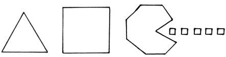
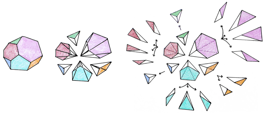
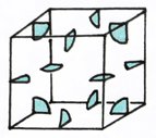
Within the constraints of this definition, polyhedra are diverse and varied. Below are some examples.
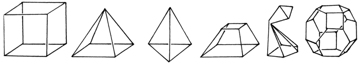
(If the squished part of the second-to-last polyhedron were further squished into a single point,
then by the third bullet point above it could no longer be a single polyhedron.)
Just as any pair of polygons of equal area can be decomposed and reassembled into the same square, can any pair of polyhedra of equal volume be decomposed and reassembled into the same cube? Are polyhedra of equal volume equidecomposable? Are they equicomplementable?
By the end of the nineteenth century there were several examples of equalvolume polyhedra that were both equidecomposable and equicomplementable, but there was no general solution. One simple example is prisms with the same height and equal area bases, stemming from the two-dimensional polygon result. In 1844 Gerling showed (and then Bricard proved again in 1896) that two mirror-image polyhedra are equidecomposable by cutting them up into congruent mirror-image pieces that can then be rotated into each other. There were also some specific tetrahedra equidecomposable with a cube, shown in 1896 by M.J.M. Hill.
We can reduce the problem about polyhedra in general to a problem about tetrahedra.
1.4 Definition III: Tetrahedron
A tetrahedron is a polyhedron with four triangular faces, six edges, and four vertices. In many current math textbooks the faces are required to be congruent. We are not going to require that any of the faces be congruent; our definition is closer to what many current math textbooks call a triangular pyramid.
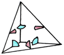
Just as any polygon can be cut up into triangles, any polyhedron can be cut up into tetrahedra. First, we can cut any polyhedron into a finite number of convex polyhedra. These can each then be cut up into a finite number of pyramids with polygonal bases. Because any polygon can be cut up into a finite number of triangles, each of these polygonal pyramids can be cut up into a finite number of triangular pyramids. This means that if we can prove or disprove the Bolyai-Gerwien theorem in the third dimension for tetrahedra, then we have also proved or disproved it more generally for polyhedra. Below is an example of a division of a polyhedron into triangular pyramids, based off of figures 13.12 and 13.13 in Rajwade’s 2001 Convex Polyhedra.
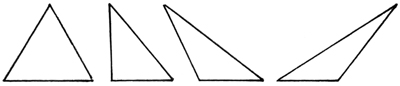
The volume of a tetrahedron is ⅓ the area of the base multiplied by the height; as described by Euclid, any two tetrahedra with bases of equal areas and with equal heights will also have the same volume. This definition of volume is reminiscent of the parallel result in two dimensions: the volume of a triangle is ½ the length of the base multiplied by the height.
Unlike the area of a triangle, however, the volume of a tetrahedron and therefore the volume of a polyhedron is found through calculus, by dividing the three-dimensional polyhedron into infinitesimally thin two-dimensional cross sections and adding up their areas.
If the Bolyai-Gerwien theorem can be expanded into the third dimension, we can define the volume of any three dimensional polyhedron the same way we define the area of a two dimensional polygon, by breaking it up into discrete building blocks—tetrahedra in three dimensions and triangles in two—and reassembling the pieces into a cube or square. This would be an elementary solution, with no infinities (or calculus) required.
This problem was posed by C.F. Gauss. In a letter in 1844, Gauss expressed that he wanted to see a proof that used finitely rather than infinitely many pieces. By Hilbert’s time it was not yet solved.
1.5 David Hilbert’s 23 Problems
One of my favorite aspects of geometry is how seamlessly it can transition from elementary school math to the cutting edge. Modern geometry is built on fluid connections between the basic principles. This foundation was built largely by David Hilbert.
The fundamentals of geometry were initially outlined by Euclid in Elements. In the nineteenth century, geometry was becoming increasingly abstract and less and less tied to the original shapes. As Hilbert said in a lecture: “One must be able to say at all times—instead of points, straight lines, and planes—tables, chairs, and beer mugs.” In this context some of the unstated assumptions in Euclid’s Elements came uncovered. (As an example, one such unstated assumption was that if two lines cross, they must have a point in common.) Hlibert extended Elements, providing an axiomization of Euclidian geometry and proofs for the unchecked assumptions that stood in the way of geometry being as fully useful as algebra.
David Hilbert was born in Wehla, Germany. His mother was interested in philosophy, and his father was a judge and wanted him to study law. He was homeschooled for two years and began school two years late, at age eight. The subject he went on to study was mathematics, because he did not like memorization.
A turning point for Hilbert was at his first presentation, at the Technische Hochschule, where he impressed and befriended Klein, 13 years his senior. After his dissertation on invariants Hilbert went to Paris to meet the leading mathematicians upon Klein’s suggestion. In his letters back to Klein, he made comical judgements of some of the most important mathematicians of the time. In particular, he reflected that Poincar´e, with whom Klein had a (mental breakdown inducing) rivalry, was quite shy, and that the reason he published a lot of papers was that he published even the smallest results.
Hilbert continued his research in Germany, first at his hometown university and then at G¨ottingen when he was invited over by Klein in 1894. In the beginning he continued to focus on invariant theory, a branch of abstract algebra examining how algebraic expressions change in response to change in their variables. Hilbert’s style of teaching was very different from Klein’s: unlike Klein’s prepared, perfectionist style of lecturing, Hilbert would prepare only an outline beforehand and work through the mathematics in front of his students, mistakes and all. Hilbert and Klein revolutionized the teaching of mathematics, incorporating visual aids and connecting mathematical concepts to their applications in the sciences, and elevated G¨ottingen to a leading institution in mathematics. It was here, starting with lectures to his students, that Hilbert became interested in geometry.
1900 was the dawning of a new century and a new era of mathematics. At the second meeting of the International Congress of Mathematicians (to this day the largest math conference, meeting once every four years, and the conference at which the Fields Medal is awarded), that year in Paris, David Hilbert, then 38, presented a monograph of ten of the open problems that he considered the most important for the next century. He published all 23 later, in a report titled simply “Mathematical Problems.” Some of Hilbert’s 23 problems have been very influential in the subsequent century of mathematics, and almost all of them have been solved. (The two that have not been solved, the axiomization of physics and the foundations of geometry, are now considered less of a priority and too vague for a definitive solution, respectively.)
1.6 Hilbert’s Third Problem
We are interested in the third of the 23 problems, which concerns the extension of the Bolyai-Gerwien theorem into the third dimension. Unlike Gauss, Hilbert did not believe that there was such a bridge: he asked simply for two tetrahedra that together formed a counterexample. Here we reproduce Hilbert’s third problem in its entirety, with the problem statement in bold.
In two letters to Gerling, Gauss expresses his regret that certain theorems of solid geometry depend upon the method of exhaustion, i.e., in modern phraseology, upon the axiomization of continuity (or upon the axiom of Archimedes). Gauss mentions in particular the theorem of Euclid, that triangular pyramids of equal altitudes are to each other as their bases. Now the analogous problem in the plane has been solved. Gerling also succeeded in proving the equality of volume of symmetrical polyhedra by dividing them into congruent parts. Nevertheless, it seems to me probable that a general proof of this kind for the theorem of Euclid just mentioned is impossible, and it should be our task to give a rigorous proof of its impossibility. This would be obtained as soon as we succeed in exhibiting two tetrahedra of equal bases and equal altitudes which can in no way be split up into congruent tetrahedra, and which cannot be combined with congruent tetrahedra to form two polyhedra which themselves could be split up into congruent tetrahedra.
Armed with our definitions, can find a more succinct and powerful statement of the challenge:
Specify two tetrahedra of equal volume which are neither equidecomposable nor equicomplementable.
Hilbert’s third problem was the first of the 23 to be solved. The first part of the problem, on equidecomposability, was solved by Hilbert’s student Max Dehn just a few months after the conference, before the full 23 problems were printed. The proof rests on a value describing a polyhedron, the Dehn invariant, which we will look at in more detail later. The Dehn invariant does not change when the polyhedron is cut apart and reassembled into a new shape: if two polyhedra are equidecomposable, then they must have same Dehn invariant (and they do). However, not all polyhedra with the same volume have the same Dehn invariant. Specifically, Dehn used the example of a regular tetrahedron and a cube of equal volume, and we will examine this case as well. Two years later Dehn showed in a second paper the second part of the problem, on equicomplementability.
An incomplete and incorrect proof was published by R. Bricard four years previously in 1896. It was not cited by Hilbert, but Dehn based his proof largely on Bricard’s.
Dehn’s paper was not easy to understand. It was refined by V.F. Kagan from Odessa in 1903. In the 1950s, Hadwiger, a Swiss geometer, together with his students found new properties of equidecomposability. This allowed for a more transparent presentation of Dehn’s proof. Further progress over the past century has made it even clearer and more concise.
We will be presenting a very recent version of the proof, published in 2010 in Proofs from the Book. You may have noticed a theme; indeed, the story of the third of David Hilbert’s 23 problems, the quest to expand or blockade the Bolyai-Gerwien theorem from the second into the third dimension, is a story of threes. We will present the solution in three parts: three definitions, three proofs, and three examples.
We have already gone through the definitions. A tetrahedron, as defined here, is a polyhedron with four (not necessarily congruent) triangular faces. Equidecomposability is a relationship between two shapes in which one can assemble one from all the pieces of another. Finally, equicomplementability is a relationship in which one can add congruent shapes to the two shapes to form two equidecomposable supershapes.
Now, we will go through the three proofs, of the pearl lemma, the cone lemma, and Bricard’s condition. Afterward we will apply the result to three example tetrahedra. Two of these tetrahedra together form a counterexample, solving Hilbert’s third problem.
2 Three Proofs
2.1 Proof I: The Pearl Lemma
Our first proof is by Benko. We start by defining the segments of an edge. Each edge in a decomposed shape consists of one or more segments that, placed end to end, make up the total length of that edge. In a decomposition of a polygon, the endpoints of segments are always vertices; in a decomposition of a polyhedron, the endpoints of segments can also be at the crossing of two edges. Otherwise, all non-endpoint points within any one segment belong to the same edge or edges. (In the decomposition of the square below, for example, the hypotenuse of the larger triangle is subdivided into two segments.)
We examine two equidecomposable figures. They are broken up into the same pieces, which are rearranged and perhaps reflected in different ways. Imagine that we must distribute whole, indivisible tokens—which we will call pearls— on all the segments in the two decompositions. The pearl lemma states that we can place the same positive number of pearls on—or, in other words, assign the same positive integer to—each segment in the two decompositions in such a way that each edge of a piece gets the same whole number of pearls no matter which of the two decompositions it is sitting in.
Below, for example, is a correct distribution of pearls on the equidecomposable house and square we looked at earlier.
For each edge of a piece, the sum of the pearls placed on the segments making up that edge in the decomposition of one figure must equal the sum of the pearls placed on the segments making up that edge in the corresponding decomposition of the other figure. In the second dimension, this simply means that the number of pearls we place on an edge in the first decomposition is equal to the number of pearls we place on that edge in the other figure’s decomposition. In the third dimension, an edge can consist of multiple segments that need not be consistent; an edge’s segments can be different, and even different in number, in the two decompositions. However, the number of pearls placed on a piece’s edge must still be the same between the two decompositions.
We can express this idea as a system of linear equations. The variables to solve for are the numbers of pearls on each segment. All of the coefficients in our linear equation are positive integers; in fact, since each segment is represented once, all of the coefficients are 1.
We can satisfy this system of linear equations by assigning a positive real number of pearls (which may or may not be an integer) to each segment. As an easy example, the number of pearls assigned to each segment can be equal to that segment’s length. Remember, though, that we cannot damage the pearls! We need to show that if our linear equation has positive real number solutions, then there are also positive integer solutions representing whole, unchopped pearls. This brings us to our second proof, a proof of the cone lemma.
2.2 Proof II: The Cone Lemma
The cone lemma is our name for the 1903 integrality argument by Kagan, which greatly simplified Dehn’s proof. We must show that if our system of linear equations has a positive real solution, then it also has a positive integer solution.
We start with a set of homogenous linear equations Ax = 0, x > 0 with integer coefficients (integer values in A) and positive real solutions (positive real values in x). This is a translation of our set of linear equations in the form Ax = b, x > 0 required by the pearl lemma. We need to show that if the set of real solutions to Ax = 0, x > 0 is not empty, then it also contains positive integer solutions.
We required that our solutions be greater than zero. However, if there are solutions that are greater than zero, then there must also be solutions greater than or equal to one, since an all-positive solution vector x can always be multiplied by some positive value to produce an equivalent vector with all values at least 1. Therefore it will suffice to show that if the set of real solutions to Ax = 0, x ≥ 1 is not empty, then it also contains integer solutions with all values greater than or equal to 1.
We will prove this using a method devised by Fourier and Motzkin. We will use Fourier-Motzkin elimination to show that there exists a lexicographically smallest real solution x to Ax = 0, x ≥ 1 and that if the coefficient matrix A is integral, then that lexicographically smallest solution is rational.
Proving that if there is a real solution, then there must exist an integer solution to Ax = 0, x ≥ 1 is equivalent to proving the same for Ax ≥ b, x ≥ 1. Therefore we will show that there exists a lexicographically smallest real solution x to Ax ≥ b, x ≥ 1 and that if A and b are integral, then that lexicographically smallest solution is rational.
(Here, the lexicographically smallest vector results from a comparison of the elements in the vectors in order. If a vector has the smallest first element, then it is the lexicographically smallest vector. If there is a tie in the first element, then we compare the second element, followed by the third, and so on.)
We will use a proof by induction on N, the size of any possible solution vector x = (x1, …, xN).
First we consider the base case, N = 1. There is only one variable x1 to solve for, and there are only inequalities that involve x1. We simply assign to x1 the smallest value that it can take on.
Now we consider solutions in multiple variables, N > 1. We examine those inequalities that involve xN. Because we have declared that all elements of the solution must be greater than or equal to 1, we know that there is at least a lower bound on xN: xN ≥ 1. There might also be additional lower bounds or upper bounds.
As before, we set xN to the smallest value it could take on. Now we are looking at a smaller system, in N − 1 variables, A’x’ ≥ b, x’ ≥ 1. This system contains all the inequalities of the previous system in N variables except for those involving xN , which we just resolved. In addition, we add a new constraint that all upper bounds on xN are at least as large as all lower bounds on xN. We continue by looking at the inequalities involving xN−1 and setting xN−1 to the smallest value it could take on, then examining xN−2, and so on.
We established that the base case system in one variable has a smallest solution. The system that preceded it is a system in two variables—we created the N = 1 system out of the N = 2 system by setting the second variable x2 to its smallest possible value. This is definitely possible to do since each variable xi has at the very least an inequality xi ≥ 1. We know then that the system in two variables has a smallest solution as well. We can follow the same logic to find that the system in three variables has a smallest solution, and a system in four variables, and so on. If the system in N variables has a smallest solution, then the preceding system in N + 1 variables has a smallest solution as well.
All of these lexicographically minimal solutions are rational, since the inequalities that we use to set the minimal value of each variable have integer coefficients.
Therefore, if a system of homogeneous linear equations has a positive real solution—as does the system generated by the pearl lemma (translated so that it is a system of homogeneous linear equations)—then it also has a positive integer solution. We have proved the cone lemma and with it the pearl lemma.
(Why is this called the cone lemma? A set of homogenous linear equations Ax = 0, x > 0 with integer coefficients—integer values in A—and positive real solutions—positive real values in x—is called a rational cone.)
2.3 Proof III: Bricard’s Condition
Our final proof allows us to connect the pearl lemma to concrete examples and finally solve Hilbert’s third problem. Bricard’s condition was claimed but incorrectly proved by Bricard in his 1896 paper. Dehn proved it successfully, and the proof has since been refined.
From here on out we will focus on the dihedral angles of three-dimensional polyhedra, the angles between faces that share an edge. A square pyramid, for example, has eight dihedral angles, one for each of its eight edges. Two of them are illustrated below
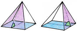
A tetrahedron has six dihedral angles (one for each of its six edges) and a cube has twelve.
Bricard’s condition states that, looking at two three-dimensional polyhedra that are equidecomposable or, more generally, equicomplementable, their dihedral angles must be linear combinations of each other with a difference of some multiple of π.
In other words, if we define the dihedral angles of one polyhedron α1, …, αr and the dihedral angles of an equidecomposable or equicomplementable polyhedron β1, …, βs, there must be some positive integers m1, …, mr and n1, …, ns and an integer k such that
m1 α1 + … + mr αr = n1 β1 + … + ns βs + kπ
We will prove first that the property holds for any two equidecomposable polyhedra and then that it holds more generally for any two equicomplementable polyhedra.
2.3.1 Equidecomposability
We start by assuming that two polyhedra are equidecomposable. As a (two-dimensional) example, we can look at the same house and square from earlier.
We cut the two polyhedra up into two decompositions made up of the same pieces, and we follow the pearl lemma to assign a positive integer number of pearls to each segment in each of the two decompositions: each piece has the same total number of pearls on each of its edges in either of the two decompositions.
At each pearl, we measure the dihedral angle made by the faces incident to the edge at the location of the perl. If the perl is in the interior of the figure, its dihedral angle will be π or 2π. If the pearl is on an edge of a piece but not on an edge of the figure being decomposed, then its dihedral angle will be π.
We define a sum ∑ 1 as the sum of the dihedral angles at all of the pearls in the pieces of the first polyhedron, one angle per pearl. We also define a second sum ∑ 2, the sum of the dihedral angles at all of the pearls in the pieces of the second shape, again one angle per pearl.
Multiple pearls can have the same dihedral angle, sometimes by being on the same edge and sometimes by being on different edges with the same dihedral angle, such as the two dihedral angles in the square pyramid illustrated earlier. In either case the dihedral angle will appear multiple times in our sum. The number of times a dihedral angle appears, and therefore its multiplier in either of the sums, must be a positive integer. Similarly, there will be an integer number of pearls with a dihedral angle of π or 2π, and therefore a nonnegative integer multiplier of π.
If we define the dihedral angles of one polyhedron α1, …, αr, we can represent the first sum as
∑ 1 = m1 α1 + … + mr αr + k1 π
for some positive integers m1, …, mr and a nonnegative integer k1.
Similarly, if we define the dihedral angles of the second polyhedron β1, …, βs, we can represent the second sum
∑ 2 = n1 β1 + … + ns βs + k2 π
for some positive integers n1, …, ns and a nonnegative integer k2.
We get ∑ 1 and ∑ 2 by adding the dihedral angles of each piece in the decompositions of the first polyhedron and the second polyhedron, respectively. These pieces are congruent, since the two polyhedra are equidecomposable and we are looking at decompositions that satisfy this relationship. Therefore by the perl lemma, which we used to distribute the pearls, each edge of each piece has the same dihedral angles in either of the two decompositions and the same number of pearls with each dihedral angle. In other words, ∑ 1 = ∑ 2 or, substituting in the definitions of ∑ 1 and ∑ 2,
m1 α1 + … + mr αr + k1 π = n1 β1 + … + ns βs + k2 π
We define the integer k = k2 − k1 and find that our equation becomes Bricard’s condition.
m1 α1 + … + mr αr = n1 β1 + … + ns βs + kπ
2.3.2 Equicomplementability
Now we assume that our two polyhedra are equicomplementable. As a two dimensional example, recall that we can add congruent pieces to our house and box—
—such that the resulting polygons are equidecomposable.
We can create two superfigures from our equicomplementable polyhedra by adding congruent pieces to the two polyhedra such that the superfigures are equidecomposable. In other words, we will be able to cut apart the superfigures so that their pieces are our two original polyhedra (one original polyhedra in each superfigure) and otherwise the same pieces. These are our first two decompositions of the two superfigures and our first decomposition of each individual superfigure. In addition, we can also cut apart the superfigures into an alternative decomposition such that they share all their pieces. These form the third and fourth decompositions of our superfigures, the second decomposition of each individual superfigure.
We again apply the pearl lemma to distribute the pearls on the edges of all the pieces in all four decompositions. Because we used the cone lemma to prove the perl lemma, we can impose an additional constraint: each edge of each superfigure must have the same total number of pearls in each of the two decompositions it is involved in.
As before, we compute the sums of the dihedral angles at all the pearls, ∑’1, ∑’2, ∑”1, and ∑”2. ∑’1 and ∑’2 are the first decomposition of each superfigure. ∑’1 includes our first original polyhedron, ∑’2 includes our second original polyhedron, and each other piece of ∑’1 is congruent to a piece in ∑’2 and vice versa. ∑”1 and ∑”2 are the alternative decompositions of the two superfigures. Each piece in ∑”1 has a congruent counterpart in ∑”2 and vice versa.
First, we notice that ∑”1 and ∑”2 are decompositions into the same pieces. As in our proof for equidecomposable polyhedra, this means that ∑”1 and ∑”2 must be identical: ∑”1 = ∑”2.
Next, we notice that ∑’1 and ∑”1 are decompositions of the same polyhedron, our first superfigure. Recall that we restricted our placement of pearls so that each edge of the superfigure needed to have the same number of pearls. Recall also that pearls that are placed inside of the superfigure or on the inside of one of its faces, rather than on one of its edges, yield dihedral angles of π or 2π. Though the two decompositions of our first superfigure might have different numbers of pearls, the edges of the superfigure itself must have the same numbers of pearls. This means that ∑’1 and ∑”1 can differ by an integer multiple of π, which we here call ℓ1.
∑’1 = ∑”1 + ℓ1 π
By the same logic, with an integer ℓ2,
∑’2 = ∑”2 + ℓ2 π
Since we deduced above that ∑”1 = ∑”2, we can restate these two equations as a relationship between ∑’1 and ∑’2, with ℓ = ℓ2 − ℓ1.
∑’2 = ∑’1 + ℓπ
We now have a statement describing the relationship between the original decompositions of the two superfigures, ∑’1 and ∑’2—we are almost done!
Remember that the difference between ∑’1 and ∑’2 is that the first contains our first polyhedron and the second contains our second polyhedron. Each other piece in ∑’1 has a congruent counterpart in ∑’2 and vice versa.
Since they are identical, we can subtract the contributions of these congruent pieces from each side of the equation. This leaves the first polyhedron’s contributions to its superfigure and the second polyhedron’s contributions to its superfigure. As before, they will differ by an integer multiple of π—ℓπ.
m1 α1 + … + mr αr = n1 β1 + … + ns βs + ℓπ
This is Bricard’s condition as described in the opening of this proof, replacing the integer k with the integer ℓ. We have now shown that Bricard’s condition holds for both equidecomposable and equicomplementable polyhedra.
2.3.3 The Dehn Invariant
We do not use it in this version of the proof, but we will pause for a moment to formally define the Dehn invariant, which was used by Dehn in his original proof. You may notice a few parallels to Bricard’s condition—indeed, though it was published earlier, Bricard’s condition is a consequence of the relationship between the Dehn invariant and equidecomposability.
We define in radians the dihedral angles of a polyhedron P: α1, α2, …, αp. We also define the lengths ℓ1, ℓ2, …, ℓp of the corresponding edges in P. The Dehn invariant f(P) of the polyhedron P with respect to the function f is the sum:
f(P) = ℓ1 f(α1) + ℓ2 f(α2) + … + ℓp f(αp)
f is an additive function—every linear dependence in the input values also exists in the output values. We also add the additional constraint that f(π) = 0.
In his original proof, Dehn showed that the Dehn invariant does not change when a polyhedron is cut apart and reassembled into a new shape: if two polyhedra P and Q are equidecomposable, then they have same Dehn invariant. In other words, for every additive function f that is defined for P’s and Q’s dihedral angles and for which f(π) = 0, f(P) = f(Q). Dehn found, however, that not all polyhedra with the same volume have the same Dehn invariant, demonstrating that not all polyhedra with the same volume are equidecomposable and thereby solving Hilbert’s third problem. This proof is more complicated than the three-part proof we presented here; it is described in detail in the corresponding chapter of the third edition of Proofs from the Book (otherwise we refer to the fourth edition).
3 Three Examples
Finally, we can apply Bricard’s condition to the dihedral angles of three example tetrahedra and identify a counterexample, our solution to Hilbert’s third problem.
3.1 Example I: A Regular Tetrahedron
Our first example is the same example used by Dehn in his first paper. Here we examine a regular tetrahedron, a tetrahedron in which each of its four faces is an equilateral triangle. All dihedral angles in a regular tetrahedron are arccos ⅓.
In contrast, all dihedral angles in a cube are π/2.
We will show that the regular tetrahedron cannot be equidecomposable nor equicomplementable with any cube. Because of the work we have already done, this is very easy to do! If a regular tetrahedron were equidecomposable or equicomplementable with a cube, then by Bricard’s condition, there must be some positive integers m1 and n1 and some integer k such that
m1 arccos ⅓ = n1π/2 + kπ
We can rearrange this equation to solve for k.
k = 1/π (m1 arccos ⅓ − n1 π/2)
k = m1 1/π arccos ⅓ − ½ n1
1/π arccos ⅓ is irrational (we will not examine the proof here, but it is in chapter 7 of Proofs from the Book). k, then, must also be irrational—it cannot be an integer. Bricard’s condition does not hold for these two figures. This means that a regular tetrahedron cannot be equidecomposable nor equicomplementable with any cube, even a cube of the same volume.
This example alone demonstrates that two polyhedra of equal volume are not necessarily equidecomposable or equicomplementable with each other. However, though we have gotten at the spirit of Hilbert’s third problem we have not solved it exactly. We will look at two more examples to produce two tetrahedra of equal volume that are neither equidecomposable nor equicomplementable.
3.2 Example II: A Tetrahedron with a Vertex Incident to Three Orthogonal Edges
Our next example very closely parallels the logic we saw above. Now we look at a tetrahedron with three orthogonal edges of equal length u that share a vertex. Three of this tetrahedron’s six dihedral angles (the turquoise angles) are right angles (size π/2). The other three (the red angles) have size arccos √⅓.
Like the regular tetrahedron in our previous example, this tetrahedron cannot be equidecomposable nor equicomplementable with a cube. If it were, then by Bricard’s condition there must be some positive integers m1, m2, and n1 and some integer k such that
m1 arccos ⅓ + m2 π/2 = n1 π/2 + kπ
As before, we can rearrange this equation to solve for k.
k = 1/π (m1 arccos ⅓ + (m2 − n1) π/2)
k = m1 1/π arccos √⅓ + ½ (m2 − n1)
1/π arccos √⅓ is irrational (this proof is also covered in chapter 7 of Proofs from the Book). As in the first example, k must be irrational as well and therefore cannot be an integer. Bricard’s condition does not hold for this relationship. This means that a tetrahedron with a vertex incident to three orthogonal edges also cannot be equidecomposable or equicomplementable with a cube.
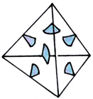
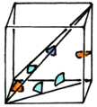
3.3 Example III: A Tetrahedron with an Orthoscheme
Finally we look at a tetrahedron with a three-edge orthoscheme: a sequence of three edges that are mutually orthogonal and in this case of identical length u, the same length as each of the three orthogonal edges in the previous example. The dihedral angles in this tetrahedron are π/2 (the three turquoise angles), π/4 (the two orange angles), and π/6 (the blue angle).
The dihedral angles of this tetrahedron are all rational multiples of π/2, the size of any dihedral angle of a cube. In fact, a cube can be decomposed into six congruent tetrahedrons with an orthoscheme.
Notice that this tetrahedron has the same base and height as the tetrahedron in the second example, and therefore the same volume. However, it cannot be eqidecomposable nor equicomplementable with a tetrahedron with those dihedral angles (or with the regular tetrahedron in the first example). If it were, then by Bricard’s condition there must be some positive integers m1, m2, m3, n1, and n2, and some integer k such that
m1 π/2 + m2 π/4 + m3 π/6 = n1 arccos √⅓ + n2 π/2 + kπ
As in the previous two examples, we can rearrange this equation to solve for k.
k = 1/π (m1 π/2 + m2 π/4 + m3 π/6 − n1 arccos √⅓ − n2 π/2)
k = ½ m1 + ¼ m2 + ⅙ m3 − ½ n2 − n1 1/π arccos √⅓
Recall from the second example that 1/π arccos √⅓ is irrational. k, then, cannot be an integer and Bricard’s condition cannot hold for this relationship. A tetrahedron with an orthoscheme of three identical-length edges cannot be equidecomposable nor equicomplementable with a tetrahedron with a vertex incident to three orthogonal edges of that same length. We have found two tetrahedra with the same base and height (and therefore the same volume) that are neither equidecomposable nor equicomplementable. In them we have found a solution to Hilbert’s third problem.
4 Open Problems
The theory of the equidecomposabililty and equicomplementability of polyhedra, revived by Hilbert’s third problem, is largely solved. When we look at polytopes in higher dimensions, however, some gaps do remain.
Though we did not use it in this proof, we mentioned earlier the Dehn invariant and its relationship with the equidecomposability of polyhedra: if two polyhedra are equidecomposable, then they necessarily have the same Dehn invariant. In 1965, Sydler proved that this condition is not only necessary, but also sufficient for equidecomposability: if two polyhedra have the same Dehn invariant, then they are necessarily equidecomposable. This result has not yet been proved—and its validity is unknown—for spheres and hyperbolic spaces of at least three dimensions, and in general for dimensions of at least five. If we only allow translations while reconstructing the second polytope from the decomposition of the first, then this problem is open in four or more dimensions.
In addition, the problem of finding the minimum number of allowed motions necessary for equidecomposability is also unsolved in four or more dimensions.
The consequences of restricting the motions in equidecomposability (to translations, to translations and central inversions, or to all motions that preserve orientation) and the existing proofs in lower dimensions are explored in depth in Boltíànskiĭ’s Hilbert’s Third Problem.
5 Conclusion
Hilbert’s third problem is one example of the necessity and beauty of a rigorous mathematical proof. If the Bolyai-Gerwien theorem could have been expanded into the third dimension, then we could define the volume of any three dimensional polyhedron using the discrete methods from the second dimension. Instead, progressing from area in the second dimension to volume in the third dimension requires breaking the shape into continuous, infinitely small building blocks and the use of calculus, an entire other toolbox and an entire other field: we share the third dimension with unavoidable infinities.
6 References
- The chapter “Hilbert’s Third Problem: Decomposing Polyhedra” (pages 53-61) from the 4th edition of Proofs from the Book by Martin Aigner and Günter M. Ziegler (published in 2010 by Springer in Berlin).
- That same chapter (pages 45-52) from the 3rd edition of Proofs from the Book (published in 2004)—this one is based on Dehn’s original proof.
- “A New Approach to Hilbert’s Third Problem” by David Benko, pages 665-76 of volume 114 of The American Mathematical Monthly (2007).
- Hilbert’s Third Problem by V.G. Boltíànskiĭ (published in 1978 by V.H. Winston Sons in Washington, D.C.).
- Polyhedra: One of the Most Charming Chapters of Geometry by Peter R. Cromwell (published in 1997 by Cambridge University Press in New York).
- Scissors Congruences, Group Homology and Characteristic Classes by Johan L. Dupont (published in 2001 by World Scientific in Singapore).
- Revolutions of Geometry by Michael O’Leary (published in 2010 by John Wiley Sons in Hoboken, NJ).
- Convex Polyhedra with Regularity Conditions and Hilbert’s Third Problem by A.R. Rajwade (published in 2001 by the Hindustan Book Agency in New Delhi).
- Hilbert’s Third Problem: Scissors Congruence by Chih-Han Sah (published in 1979 by Fearon Pitman in San Francisco).

If you’re hungry for more college-level math, I recommend starting with Proofs from the Book, the source of this proof and the textbook we used in 18.304—they just came out with their fifth edition and you can read it for free online. Proofs is divided into five sections, each one containing a sample of a field of mathematics: number theory, geometry, analysis, combinatorics, and graph theory. Together these cover a lot of what we learn in course 18 and, in the case of combinatorics and graph theory, course 6-3 (or the course 6 part of 6-7, in my case).